- Coffee House Post #3, Published online on 23rd April 2020
- Noelia Iranzo Ribera is a 2nd year PhD researcher at the University of Birmingham working on causal modelling and the metaphysics of causation in physics. She holds a BSc in physics, but her current areas of interest are philosophy of science and philosophy of physics. In particular, during her dissertation she aims to develop an account of laws and causal models that can be used by philosophers and physicists alike. She is part of the FraMEPhys project, funded by an ERC Starting Grant: https://framephys.org.
Quantum entanglement is the defining feature of quantum mechanics. As Erwin Schrödinger once wrote, it is “the characteristic trait of quantum mechanics, the one that enforces its departure from classical lines of thought” (Schrödinger 1935, p. 555). But in which sense does quantum entanglement depart from classical lines of thought? The common answer is that it brings about the existence of non-local correlations,[1] and non-locality is a double-edged phenomenon; while it can be tapped for the benefit of quantum computing purposes, it is at odds with the theory of relativity. In this entry I will argue that quantum entanglement’s departure from locality is not its only peculiar feature; the apparent impossibility to give a causal explanation of entanglement statistics even if non-locality is assumed should strike us as equally puzzling. If quantum entanglement is an empirical phenomena, how come we cannot infer causal lessons from such correlations as we do elsewhere in our scientific endeavors? Does such a negative result call for a revision of the principles guiding our causal inferences?
1. EPR/B Systems, Bell’s Theorem and Entanglement Statistics
More than half a century after its publication, and due to divergences in its interpretation, Bell’s theorem is still one of the most debated topics in the philosophy of physics. Assuming a local and classical worldview, the theorem derives an upper limit for the strength of correlations between distant events, a limit which is violated by outcomes of experiments with entangled objects. In its initial formulation (Bell 1964), the theorem relied on quantum-mechanical predictions for the correlations, since experiments on entangled quantum systems had not yet been carried out, and thus it was not clear whether it was the calculations that were erroneous or one or more of the assumptions untenable. Experimental research on pairs of entangled photons led by French physicist Alain Aspect (Aspect, Dalibard and Roger 1982) and ensuing refinements and variants of such experiment confirmed that, unless one were skeptical of scientific practice/methodology, our theorizing had been slightly misguided. Most scholars agree that Einstein’s locality assumption that causal influences obey relativistic constraints (Einstein, Rosen, Podolsky 1935 –EPR hereafter) is violated in the quantum world, but that cannot be the end of the story: a violation of the locality assumption does not imply that a causal explanation of the phenomenon can be given. Quite the opposite; causal assumptions remain troublesome, and so do the observed correlations between measurement outcomes on entangled states, which are left unexplained.
Quantum entanglement is a physical phenomenon exhibited by pairs or groups of particles such that the quantum state of each particle cannot be described independently of the state of the others; it is for this reason that they can only be characterized by superpositions of product states. For the sake of simplicity and historical accuracy we will focus on bipartite entangled quantum systems, e.g. pairs of spin one-half particles in the singlet state and moving freely in opposite directions (as in Bell’s original derivation), or the equivalent pairs of photons with entangled polarization states that are often used in the experimental tests of the Bell’s inequalities. Given that in the derivation of the infamous inequality Bell used Bohm’s and Aharonov’s reconstruction of the EPR thought experiment (EPR 1935, Bohm and Aharonov 1957), in the philosophy literature these experiments are commonly referred to as EPR/B experiments.
Consider the following rotationally symmetric entangled polarization Bell state:
| ψ >= 1/21/2(|+z>1)|-z>2 – |-z>1 |+z>2 ) (1)
Where “|+z>” stands for polarization along the z-direction, and “|-z>” represents a polarization perpendicular to z. As said, a source emits photons in opposite directions towards two polarization-measurement devices A and B, which have pointers that adjust the direction (angle) in which the polarization is measured, respectively represented by a and b. When a photon arrives at the measurement apparatus, the apparatus detects whether the photon is polarized along the chosen direction (+) or perpendicular to it (-). We will represent the outcome at detector A by the variable α, and the outcome at detector B by the variable β, each of which can take one of the two possible values, “+” or “-.” Upon measurement of the polarization states of the photons, the outcomes appear to be correlated (to some, different degrees)[2] regardless of the measurement settings. That should strike us as odd, since i) the measurement settings are chosen randomly and independently of each other, and ii) the measurement settings do not depend on the entangled state ψ at the source –actually, in stringent versions of the experiment, the measurement settings are chosen after the photons have been emitted, and so according to the theory of relativity, a and b cannot be in ψ’s causal past (Näger and Stöckler 2018, pp. 121-124). Graphically, the situation is the following:
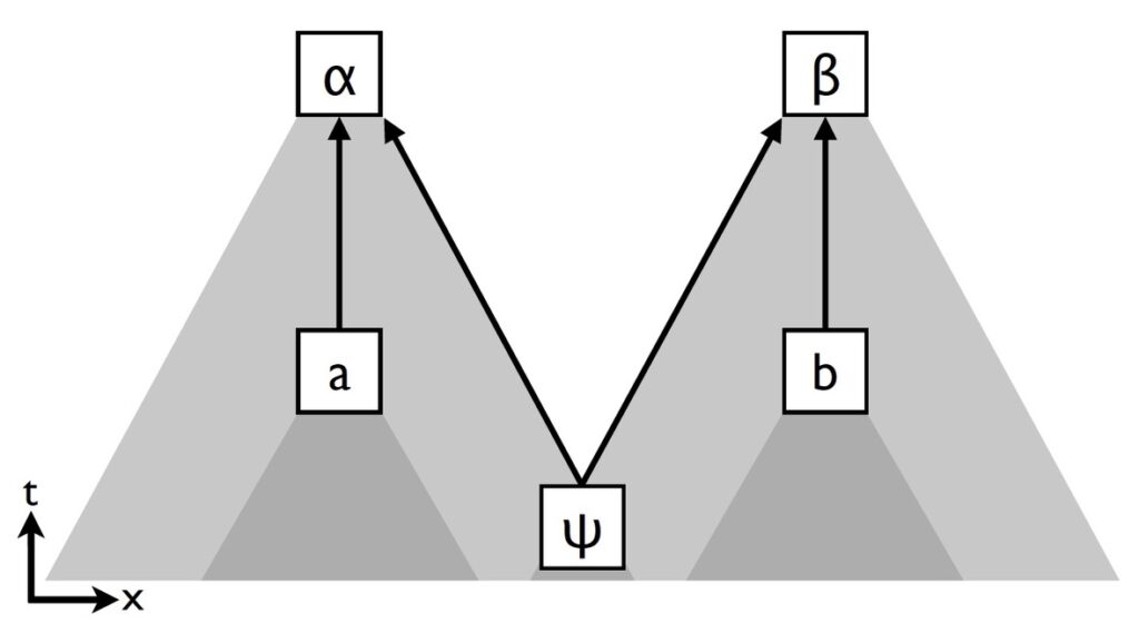
Fig. 1. Local causal graph of an EPR/B experiment, in Näger and Stöckler (2018, p. 126).
Fig. 1 is a local causal graph of an EPR/B experiment. Arrows represent causal connections, and variables represent properties of objects or events. The grey areas are the past light-cones of the five events considered above. The assumption of locality –also called ‘causal connectibility’– or the idea, in line with the main principle of the theory of relativity, that causal influences cannot travel faster than the speed of light, is made apparent. What the graph in fig. 1 tells us is that the polarization states α and β[3] can only be influenced by anything in their past light cone; in this case, ψ. This relativistic constraint also underlies Reichenbach’s Principle of the Common Cause (Reichenbach 1956): if two events X and Y are correlated but none of them causes the other, then the correlation is due to a common cause Z that renders them conditionally independent. As an example, consider the following scenario: there seems to be a positive correlation between eating ice-creams and hypothermia. “How nonsensical!,” you might exclaim. Indeed, such correlation disappears once one considers that hot weather might be the common factor causing both increase in ice-creams intake and hypothermia cases.
As mentioned, Bell (1964) ‘used’ a similar setup where the source did not emit photons but spin one-half electrons, and Stern-Gerlach apparatuses played the role of the polarization detectors of the example just considered. In Bell’s thought experiment, the locality assumption is incorporated by assuming a spacelike distance between Stern-Gerlach devices. Crucial in his derivation is that ψ does not necessarily refer to the quantum-mechanical wave-function, described by specific dynamics. A later and more general version of Bell’s proof (Bell, 1975) actually considers the possibility that the wave-function does not fully describe the entangled state, and so incorporates an empirically inaccessible or ‘hidden’ variable λ acting as an additional common cause in the causal structure of fig. 1 –see fig. 2 below. As it’s well known, Bell’s theorem applied to such improved structure tells us that no theory with hidden variables (HVT) which reproduces the predictions of quantum mechanics can be local.
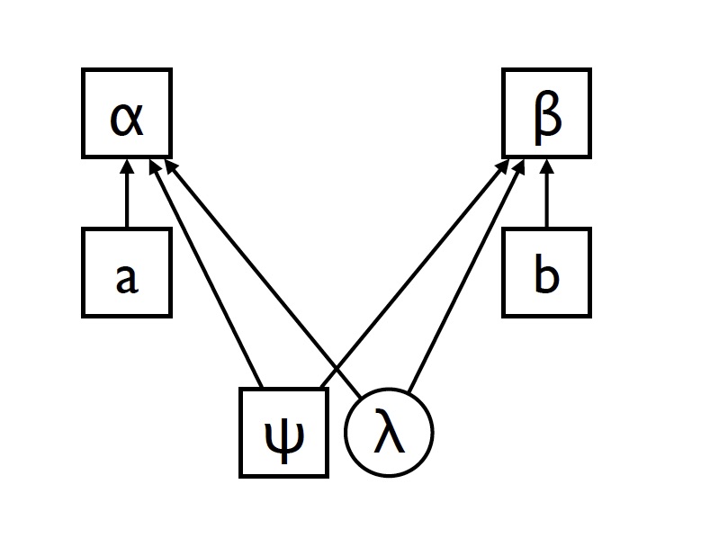
Fig. 2. Local causal structure with hidden variables in Näger and Stöckler (2018, p. 132).
An important feature of Bell’s theorem is that although his first derivation (Bell 1964) assumed determinism and perfect (anti)correlations between measurement outcomes, it can be derived from much weaker assumptions; Clauser et al. (1969) derived a Bell inequality –the famous CHSH inequality– without assuming perfect correlations and that determinism need not be assumed in the derivation (Bell 1975). It is actually the stochastic generalisation of Bell’s theorem (Clauser et al. 1969, 1974; Bell 1975) that will be of our interest in the following section.
2. Local Causality, Factorizability, and the Causal Markov Condition
Bell’s notion of local causality, crucial in his derivation of the inequality for both deterministic (Bell 1964) and stochastic theories (Bell 1975), deserves some conceptual scrutiny. In the stochastic version, Bell advanced a theory of be-ables –term to refer to entities corresponding to something real (Bell 1990, p. 234)– localized in regions in space-time, in which the assignment of values to beables implies a probability distribution for other beables. Say A and B are spacelike separated beables ( Δs2 ) located in two different spacetime regions 1 and 2, M and O the beables in the past light cones of A and B, being N the complete specification of the beables in the overlap of their light cones.
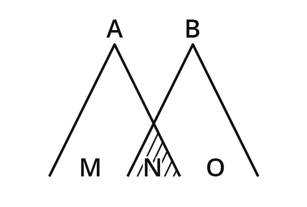
Fig. 3. Beables diagram. A is a beable in spacetime region 1, and B a beable in spacetime region 2. N is the complete specification of beables in the overlap of the light cones of A & B. M & O are beables in the remainders of the two backward light cones.
The joint probability distribution for A and B is:
P(A,B|M,N,O)=P(A|M,N,O,B)P(B|M,N,O) (2)
Where (2) follows from the product rule in probability theory. In a locally causal theory (Bell 1971, p. 54):
P(A|M,N,B)=P(A|M,N) (3)
From (2) and (3) we get Bell’s factorizability condition:
P(A,B|M,N,O)=P(A|M,N) P(B|N,O) (4)
How does Bell justify equation (3)? With respect to local causality, Bell writes (Bell 1971, p. 54):
“Now my intuitive notion of local causality is that events in 2 should not be ‘causes’ of events in 1, and vice versa.”
Where 1 and 2 are labels for spacelike separated regions. Or as he would later on write in ‘La Nouvelle Cuisine’ (Bell 1990, p. 239):
“The direct causes (and effects) are near by, and even the indirect causes (and effects) are no further away than permitted by the velocity of light.”
He turned these intuitions into the probabilistic assumption (3), crucial in the derivation of the local factorizability condition for the joint probability distribution for A and B (4). The important point here is to realize that local causality is a notion arising from physical intuitions, whereas the resulting factorization condition is a mere statistical tool –a screening off probabilistic principle. The factorization or screening off principle applied to the causal structure in fig. 2 takes the following form:
P(αβ|abψλ) = P(α|aψλ) P(β|bψλ) (5)
Which is none other than an application of Reichenbach’s Principle of the Common Cause. The probability distribution factorizes because measurement outcomes α and β are not direct causes of each other, so correlations between them can only arise because of a common cause in the overlap of their past light cones. This is a special case of the Causal Markov Condition (CMC), which is a central methodological or translation principle in recent literature on causal inference from statistical data (Spirtes, Glymour, Scheines 2000; Pearl 2000) and as such enables us to read conditional probabilities as referring to causal connections. In particular, the CMC says that the conditional probability of a variable in our model is only sensitive to its direct causes. For this reason, the CMC is the central causal assumption in Bell’s theorem.
However, there are other causal assumptions that should be made explicit. The second is that causation’s arrow follows that of time; causation is asymmetric and moves in the forward direction of time. This implicit assumption can also be stated as the idea that backwards causation or retrocausality is disallowed.
The third assumption is the ‘intervention’ assumption, which incorporates observations i) and ii) in section 1. This assumption is that the choice of measurement settings (e.g. the polarizer settings) and the quantum state are uncaused –and in this sense, free or exogenous– variables. This exogeneity is crucial, not only for its implication that the choice of settings does not affect the preparation of the quantum state, but also because since these variables cannot be influenced by any hidden variable λ this intervention assumption translates to the statistical condition that the conditional probability of λ on other variables reduces to its marginal probability.
The last assumption, and as it’s clear from Bell’s second quote above (Bell 1990, p. 239), is that the boundaries of causal connectibility correspond to the null cone structure of Minkowski space-time (E.g. Brown and Timpson 2016, p. 14). That no super-luminal signalling plays a significant role in defining local causality is a point that has been properly acknowledged in the philosophical literature on Bell’s theorem. However, what I have tried to show in this section is that there are other causal assumptions behind it, and that these should be made precise.
The factorizability condition (5) thus formalizes the idea that measurement outcomes can only be influenced by the measurement setting in their respective wing of the experiment, the quantum state at the source, and the hidden variables. Or as Jarrett (1984) and Shimony (1984) have shown, the factorization condition is a combination of two statistical independence conditions:[4]
- Conditional outcome independence (OI): the probability determined for a certain outcome at one measurement setting is invariant under conditionalization on the outcome at the other measurement setting.
- Parameter independence (PI), also referred to as ‘no-signalling’ condition: the marginal probabilities of measurement outcomes do not depend on the settings of the distant apparatuses.[5]
OI and PI play a prominent role in discussions about the conflict between non-locality and relativity theory; the vast majority of authors advocate a failure of non-locality as the correct interpretation of Bell’s theorem explainable by a failure of OI above –as hinted by the empirical outcome dependence observed in real experiments.[6]
The literature on Bell’s theorem and quantum entanglement has made it explicit that a failure of non-locality is problematic in two respects. First, it conflicts with relativity theory. There are many reasons why the theory of relativity forbids superluminal causal influences, an important one being that they lead to self-contradictory signal loops. Second, it is an empirical fact that in EPR/B experiments signals cannot be sent at speeds greater than that of light. Näger (2016) has dubbed this traditional take on the problem ‘the spatiotemporal problem of entanglement.’[7]
3. The Causal Problem of Entanglement
Setting the relativistic concerns aside, there is an additional incongruence with respect to quantum entanglement: whether one can explain its rather awkward statistics through a causal (or, as we will see in section 5, even non-causal) structure and some appropriately motivated principles. This diagnosis has recently been made by Wood and Spekkens (2015) and more emphatically by Näger (2016), and has been named ‘the causal problem of entanglement’ (CaPrEnt hereafter) by the latter author. While we have been implicitly introducing some of these ideas throughout this entry, the CaPrEnt can be more clearly formulated as the inconsistency between the following in EPR/B experiments:
- EPR/B statistics, empirically confirmed by Stuart J. Freedman & John F. Clauser (1972) and Alain Aspect et al. (1982).
- Locality, or the requirement that causal influences between physical systems propagate subluminally.
- Causality, or principles of causal explanation –to be detailed shortly.
The problem is then that, even if one accepts that non-local influences hold between distant measurements, the measurement statistics of entangled quantum systems is per se in conflict with the usual principles of causal explanation (Näger 2016). In other words, a tension with the causality requirement above remains regardless of our withholding or giving up of the locality requirement; even if we accept some form of non-locality, a causal explanation of EPR/B entanglement scenarios cannot be given.
The relationship between requirements i. and iii. above can be made more explicit with the use of the theory of causal graphs, also known as causal Bayesian networks. Causal graphs (like those of figs. 1 & 2) are used in many fields (e.g. statistics, econometrics, epidemiology, philosophy, etc.) as ‘devices’ representing causal relations, as well as tools to infer causal relationships from statistical data. Given that there is plenty of statistical data available for EPR experiments, there is reason to believe causal graphs might successfully represent and explain the correlations observed in quantum entangled systems. Causal graphs are subjected to the following axioms:[8]
- They are directed and acyclic (DAGs). A directed graph G corresponds to a set of vertices and a set of directed edges among the vertices. Acyclicity is the requirement that there are no directed causal paths that begin and end at the same vertex (Wood and Spekkens 2015, p. 4)
- The Causal Markov Condition (CMC). The conditional probability of a variable in a causal model is only sensitive to its direct causes. It can also be stated as the condition that every statistical dependence implies a causal dependence.
- The Causal Faithfulness Condition (CFC), also known as ‘stability’ (Pearl 1988b) and ‘no fine-tuning’ (Evans 2018). Only those independencies allowed by the CMC are allowed; in other words, every statistical independence implies a causal independence.
Restated in terms of the theory of causal graphs, the CaPrEnt discloses a tension with (at least) one of these axioms. The question now is: would abandoning (at least) one of them explain the statistics observed in EPR/B experiments?
4. Is There a Way Out?
In this section we shall examine what a failure of each of the conditions listed in the previous section would amount to.
- A Failure of the DAG mode of representation: Under this category, one ought to consider a failure of directedness and/or acyclicity. A failure of directedness would leave the doors open to the possibility of backwards causation. Acyclicity would allow causal feedback loops, a move which, as mentioned, raises concerns.
- Retrocausation: the possibility that causal influences do not follow the standard arrow of time. E.g. Price (2001, 2008) has a model for backwards causation that rests on abandoning the idea that hidden variables are independent of future measurement settings. Nonetheless, Wood and Spekkens (2015, p. 22) argue that even for retrocausal models fine-tuning of the causal parameters would be needed.
- A Failure of the CMC: It is the central methodological assumption of all empirical sciences that correlations require explanation –only if we understand the (in this case, causal) origin of correlations we can exploit these relationships between events or properties for control and predictive purposes. By giving up the CMC there would be no way of attaching probability distributions to DAGs, and so under which circumstances a certain connection implies which statistical facts would become an epistemic impossibility. Abandoning the CMC is thus a threat to statistical modelling as a whole. Failures of the CMC in the quantum realm have been advocated by Glymour (2006).
- A failure of the CFC: A priori nothing rules out the possibility of a causal dependence relation that appears as a statistical independence relation. Some authors (See Wood and Spekkens 2015, Näger 2016, and Evans 2018 for full proposals) have defended that failures of the CFC are permitted as long as they are stable. Cartwright (2007) and Andersen (2013) have discussed macroscopic violations of the CFC, and Frisch (2014) has also argued for the feasibility of fine-tuned causal models in experimental physics. While being the most popular solution, it is difficult to see how the existence of a causal influence that does not leave any trace in the statistics could be of use to the experimental physicist.
Alternatively, and while acknowledging that judging measurements to have been performed erroneously would be a contentious solution, one could also adduce to:
- A failure of the Intervention Assumption: Also known as the freedom-of-choice loophole (Bell 1975, 1977, Shimony 1976). Part of everyday experimental practice, ruling it out would be an ad hoc solution leading to some kind of superdeterminism or cosmic conspiracy according to which experimenters have no free will or freedom of choice, no control over the setup of experiments.
5. Beyond Causal Explanation
A crucial but under-looked point with respect to the analysis in section 3 is that the so-called CaPrEnt does not only affect causal connections, but also any kind of non-causal connection that claims to explain statistical facts. According to Näger and Stöckler (2018, pp. 165-167), whatever non-local kind of connection between measurement outcomes there is, it would have to:
- Produce the observed correlations between measurement results.
- Not produce the observed correlations, in order to prevent the superluminal transmission of signals –and so satisfy the no-signalling condition.
Even if one is convinced that having one of the failures detailed in the previous section is a sign of an impossibility to give a causal explanation of quantum entanglement, and resorts instead to, say, some other type of non-local non-causal metaphysical connection between measurement outcomes (e.g. a state-of-the-art grounding relation such as the one proposed by Ismael and Schaffer (2016)),[9]: a difficulty persists in making such relation accountable for the observed correlations and independencies. Even when interpreted as a non-local non-causal phenomenon, quantum entanglement’s queerness keeps fascinating all sorts of crowds.
References
Andersen, Holly. 2013. “When to Expect Violations of Causal Faithfulness and Why it Matters,” Phil. Sci. 80 (5): 672-683.
Aspect, Alain. Dalibard, Jean, and Roger, Gérard. 1982. “Experimental test of Bell’s inequalities using time-varying analyzers,” Phys. Rev. Lett. 49: 1804-1807.
Bell, John S. 1964. “On the Einstein-Podolsky-Rosen paradox,” Physics 1 (3): 195-200.
Bell, John S. 1975. “The theory of local beables,” TH-2053-CERN. Reprinted in Speakable and Unspeakable in Quantum Mechanics: Collected Papers on Quantum Mechanics, 52-62. 1987. Cambridge: Cambridge U.P.
Bell, John S. 1977. “Free variables and local causality.” Epistemological Letters. 15: 79-82. Reprinted in Speakable and Unspeakable in Quantum Mechanics: Collected Papers on Quantum Mechanics, 100-104. 1987. Cambridge: Cambridge U.P.
Bell, John S. 1990. “La nouvelle cuisine.” In Speakable and Unspeakable in Quantum Mechanics: Collected Papers on Quantum Mechanics, 232-248. 2004, Second Edition (1st edition: 1987). Cambridge: Cambridge U.P.
Bohm, David and Yakir Aharonov. 1957. “Discussion of Experimental Proof for the Paradox of Einstein, Rosen, and Podolsky,” Phys. Rev. 108 (4): 1070-1076.
Brown, Harvey R. and Christopher G. Timpson. 2016. “Bell on Bell’s Theorem: The Changing Face of Nonlocality.” In Quantum Nonlocality and Reality: 50 Years of Bell’s Theorem, edited by Mary Bell and Shan Gao, 91-123. Cambridge: Cambridge U.P.
Cartwright, Nancy. 2007. Hunting Causes and Using Them. Cambridge: Cambridge U.P.
Clauser, John, Michael A. Horne, and Abner Shimony. 1969. “Proposed experiment to test local hidden-variable theories,” Phys. Rev. L. 23 (15): 880-884.
Clauser, John, Michael A. Horne, and Abner Shimony. 1974. “Experimental consequences of objective local theories,” Phys. Rev. D. 10 (2): 526-535.
Einstein, Albert, Boris Podolsky, and Nathan Rosen. 1935. “ Can the quantum-mechanical description of physical reality be considered complete?,” Phys. Rev. 47:777-780.
Evans, Peter. 2018. “Quantum Causal Models, Faithfulness, and Retrocausality,” Brit. J. Phil. Sci. 69: 745-774.
Frisch, Mattias. 2014. Causal Reasoning in Physics. Cambridge: Cambridge U.P.
Glymour, Clark. 2006. “Markov properties and quantum experiments.” In Physical theory and its interpretation: Essays in honour of Jeffrey Bub, edited by William Demopolous and Itamar Pitowsky, 117-125. Dordrecht: Springer.
Howard, Don. 1989. “Holism, separability, and the metaphysical implications of the Bell experiments.” In Philosophical Consequences of Quantum Theory: Reflections on Bell’s Theorem, edited by James T. Cushing and Ernan McMullin, 224-253. Notre Dame: University of Notre Dame Press.
Ismael, Jennan and Jonathan Schaffer. 2016. “Quantum holism: nonseparability as common ground,” Synthese: 1-30.
Jarrett, Jon P. 1984. “On the Physical Significance of the locality conditions in the Bell arguments,” Noûs 18: 569-590.
Näger, Paul M. 2016. “The Causal Problem of Entanglement,” Synthese 193 (4): 1127-1155.
Näger, Paul M. and Manfred Stöckler. 2018. “Entanglement and Non-locality: EPR, Bell, and Their Consequences.” In The Philosophy of Quantum Physics, by Cord Friebe, Meinard Kuhlmann, Holger Lyre, Paul M. Näger, Oliver Passon, and Manfred Stöclker, 103-178. Translated by William D. Brewer. Berlin: Springer.
Pearl, Judea. 1988b. Probabilistic Reasoning in Intelligent Systems. San Francisco: Morgan Kaufmann.
Pearl, Judea. 2000. Causality: Models, Reasoning, and Inference. Cambridge: Cambridge U.P.
Price, Huw. 2001. “Backwards causation, hidden variables and the meaning of completeness.” Pramana 56, 199-209.
Price, Huw. 2008. “Toy models for retrocausality.” Stud. Hist. Phil. Sci. B. 39: 752-761.
Reichenbach, Hans. 1956. The Direction of Time. Berkley: University of California Press.
Redhead, Michael L.G. 1987. Incompleteness, Nonlocality, and Realism: A Prolegomenon to the Philosophy of Quantum Mechanics. Oxford: Clarendon Press.
Schrödinger, Erwin. 1935. “Discussion of probability relations between separated systems.” Math. Proc. Camb. Philos. Soc. 31 (4): 555-563.
Shimony, Abner, John F. Clauser, and Michael A. Horne. 1976. “Comment on Bell’s Theory of Local Beables,” Epistemological Letters 13: 1-8.
Shimony, Abner. 1984. “Controllable and uncontrollable non-locality.” In Foundations of Quantum Mechanics in the Light of New Technology, ed. S. Kamefuchi, 225-230. Tokyo: The Physical Society of Japan.
Spirtes, Peter, Clark Glymour, and Richard Scheines. 2000. Causation, Prediction, and Search. Second Edition (1st edition: 1993). Cambridge, MA: MIT Press.
Teller, Paul. 1986. “Relational holism and quantum mechanics,” Brit. J. Phil. Sci. 37: 71-81.
Wood, Cristopher J. and Robert W. Spekkens. 2015. “The lesson of causal discovery algorithms for quantum correlations: causal explanations of Bell-inequality violations require fine-tuning,” New J. Phys. 17: 1-29.
[1] While all pure entangled systems exhibit non-local dependences, there are mixed entangled states (e.g. Werner states) that are Bell-inequality-satisfying. Entanglement is a necessary but not sufficient condition for non-locality; the sufficient condition is that a Bell inequality is violated.
[2] Perfect correlations of measurement outcomes when measurement settings are parallel, and correspondingly weaker correlations when the settings are rotated relative to each other.
[3] Note that α and β are not polarization states; rather, they represent polarization states. For simplification purposes, talk of variables will be used to refer to the thing being represented.
[4] The names are due to Shimony (1984). Jarrett (1984) used the names ‘completeness’ and ‘locality’ to respectively refer to OI and PI.
[5] Probabilistic analogue of the locality assumption in Bell’s 1964 paper, in which he derived an inequality for deterministic theories.
[6] In this standard view, the idea is that the influence between outcomes is either non-causal (Shimony 1984, Redhead 1987) or a holistic non-separability (Howard 1989, Teller 1986, Shimony 1984, Redhead 1987).
[7] It is good to bear in mind that the no-signalling theorem in quantum mechanics prevents there from being a direct conflict with special relativity; in other words, quantum mechanics conflicts with the spirit but not the letter of special relativity.
[8] This is not an exhaustive list. Sometimes other axioms are listed: e.g. a minimality condition, a sufficiency condition, etc.
[9] In analytic philosophy, a grounding relation is a type of metaphysical relation. E.g. there is a grounding relation between a water molecule and its hydrogen and oxygen atoms. Such relation has two important characteristics. First, it’s explanatory; the existence of the atoms explains the molecule’s existence. Second, it’s a priority relation; the existence of the atoms is prior to the existence of the molecule.