- Coffee House Post #2, Published online on 31st March 2020
- About the author: Tiziano D’Albis is a postdoctoral researcher in computational neuroscience at Humboldt Universitaet zu Berlin. With a background in computer engineering, he is particularly interested in mechanisms for learning and memory and synaptic plasticity in the brain. For his doctoral thesis, he developed a model for the origin of grid-cell activity in the entorhinal cortex. A list of publications is available on Google Scholar
When we visit a new environment – such as a foreign city – we are initially disoriented. To find our way to a museum or a local restaurant we need to rely on printed maps from the tourist kiosk or electronic maps on our smartphones. Yet, with experience, we are soon able to recognize previously encountered routes and landmarks and even get back to our hotel taking detours and shortcuts. But how do we acquire spatial knowledge?
And how is physical space represented in the brain?
The cognitive map theory
A prominent theory in experimental psychology posits that men and other animals can interiorize spatial experiences in a sort of ‘cognitive map’ of the environment, i.e., a mental representation of space that embeds known places and their relations into a common reference frame (Tolman, 1948). For example, when a friend asks for directions to our home, we can create a mental image of the roads, turning points, and landmarks along the way. This representation is a cognitive map.
The cognitive-map theory was introduced by the psychologist Edward Tolman to explain rodents’ spatial behavior (Tolman, 1948). Tolman himself cites an anecdote reported by Karl Lashley in 1929. He once discovered that some rats, after having learned a maze, they “pushed back the cover near the starting box, climbed out and run directly across the top to the goal box where they climbed down again and ate” (Tolman, 1948). Such a behavior was in striking contrast to the common belief at the time that rodents simply use stimulus-response associations to solve mazes – alike to learning the right connections in a complicate telephone switchboard. In fact, through a series of ingenious experiments, Tolman (1948) demonstrated that rats’ spatial behavior resembled more a sophisticated control room than an old-fashioned telephone exchange. Tolman writes: “in the course of learning something like a field map of the environment gets established in the rat’s brain” (Tolman, 1948).
Place and grid cells
Tolman’s cognitive map, however, remained a purely theoretical concept for many years. It was not until O’Keefe and Dostrovsky (1971) discovered place cells in the hippocampus (one of the phylogenetically best preserved structures of the mammalian cortex) that neural correlates of space were first observed in experiments. By recording from the dorsal hippocampus of freely-moving rats, O’Keefe and Dostrovsky (1971) found neurons that responded “solely or maximally when the animal was situated in a particular part of the testing platform”. These neurons – which are now called place cells – were immediately seen by the experimenters as the neural substrate of the cognitive map theorized by Tolman more than twenty years earlier.
With the discovery of hippocampal place cells, a high-level cognitive concept – such as the perception of one’s location in the environment – could be studied for the first time at a mechanistic level, thereby bridging a large gap between psychology and physiology.
Thirty-four years after place-cell activity was first reported, another major breakthrough was made in the field of systems neuroscience. In a quest of unveiling the inputs to the hippocampus, Hafting et al. (2005) recorded neural activity in the medial entorhinal cortex (MEC) – a crucial anatomical hub at the interface between the hippocampus and the neocortex. In this region, neurons with remarkable spatial representations have been discovered: the grid cells. Grid cells, like place cells, activate accordingly to the position of the animal in the enclosure; however, unlike place cells, a single grid cell fires at multiple spatial locations that tile the environment with a strikingly-regular triangular pattern (Figure 1).
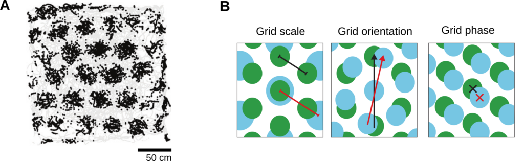
Grid cells in the entorhinal cortex. A) Spatial firing pattern of a grid cell recorded in the rat’s entorhinal cortex. The gray trace shows the trajectory of the animal foraging in a square enclosure. The black dots indicate the locations at which the cell fired. B) Illustration of the three fundamental properties of grid patterns. The grid scale (left) is the distance between two neighboring firing fields. The grid orientation (middle) is the angle between one of the grid axis and a reference direction. The grid spatial phase (right) is the spatial offset between the firing fields and a reference point. Images in panels A and B are adapted from (Moser et al., 2014) with permission from Nature Publishing Group.
Grid-cell activity was shown to represent space with a remarkably efficient code (Wei et al., 2015; Stemmler et al., 2015) – which no theorist had previously predicted to be implemented in the brain. To date, however, the mechanisms underlying the origin of grid-cell patterns are yet to be understood.
How do grids emerge in the brain?
An intresting theory for the emergence of grid-cell activity was put forward by Kropff and Treves (2008). The authors proposed that spatially-periodic patterns could arise in single neurons via three simple ingredients: 1) spatially-selective inputs; 2) Hebbian synaptic plasticity; and 3) spike-rate adaptation (Figure 2A).
Spatially-selective inputs are cells that are tuned to the physical location of the animal but do not display any particular spatial patterning – such cells are abundant in the MEC and its afferent structures (Diehl et al., 2017).
Hebbian synaptic plasticity, often exemplified by the motto: “fire together wire together”, is a physiological mechanism by which the connections (synapses) between two neurons are strengthened if their activity is correlated – a phenomenon that is ubiquitous in the brain (Citri and Malenka, 2008). Finally, spike-rate adaptation is an intrinsic cellular or synaptic process that hinders a neuron to fire for long stretches of time – a sort of safety break that reduces output firing in case of sustained and prolonged excitation (La Camera et al., 2006).
Here is an intuition of how these three ingredients may generate grid-like patterns (Figure 2B). As the animal traverses an input firing field (orange disk), the output neuron starts firing and the synaptic weight of the associated pre-synaptic neuron is potentiated by the plasticity rule. After a short time, however, the output neuron may reduce or even cease firing due to to its intrinsic spike-rate adaptation mechanism. As a consequence, the output-neuron activity is now uncorrelated to the one of inputs with fields in a ring of locations around the last activation (blue ring) and the corresponding synapses are depressed. Finally, as the output neuron recovers from adaptation, input-output activities return correlated and trigger the potentiation of new synapses (orange disk outside the blue ring). In such a learning process, the output neuron slowly develops firing fields that are separated by a typical length scale, which depends on the recovery time of adaptation and the average exploration speed of the animal. Assuming isotropic spatial exploration (i.e., roughly circular adaptation rings), an optimal equilibrium in terms of coverage is obtained when the output fields are arranged in a lattice of equilateral triangles (Figure 2C; Thue, 1910) -a configuration that is reminiscent of grid-cell patterns (Hafting et al., 2005).
In the following, I show that the idea described above can be formalized in a computational model that generates grid-like activity in numerical simulations. To this end, I introduce the model described in (D’Albis and Kempter, 2017), which builds upon the original work of Kropff and Treves (2008) by improving biological plausibility and allowing for analytical treatment. Note that many other alternative grid-cell models have been be proposed, see e.g. (Giocomo et al., 2011; Zilli 2012) for reviews.
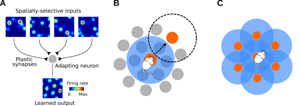
Theory for the emergence of grid-patterns A) Schematics of the model architecture. A single cell (gray disk) receives synaptic input from spatially-tuned neurons. Input spatial-tuning maps are shown at the top. B) Illustration of the pattern-formation mechanism. Input firing fields are denoted by gray disks. The orange disk at the center denotes an input firing field at the current location of the animal. At this location, the output neuron fires and active inputs are potentiated by the synaptic plasticity rule. After a short time, the output neuron decreases firing due to spike-rate adaptation, i.e., the neuron is less active within an ‘adaptation ring’ around the current location of the animal (blue ring). After recovery from adaptation, the animal has moved outside the adaptation ring, and a new input-output association can be learned (orange disk outside the blue ring). The dashed circle denotes the next adaptation ring. C) Illustration of a possible equilibrium of the learning process. The hexagonal packing is a theoretical optimum.
Modeling the origin of grid-cell patterns
Let us consider a single output neuron that receives input from N excitatory cells (Figure 2A). Input spikes are generated randomly (inhomogeneous Poisson process) with firing rates that are tuned to the location of a virtual rat. Similarly, output spikes are generated by an inhomogeneous Poisson process with rate

where r0 is a baseline firing rate, w i is the synaptic weight of input neuron i, and the function K is a temporal filter modeling spike-rate adaptation (Figure 3A). Intuitively, at the arrival of an input spike, the firing probability of the output neuron is first increased for a short time and then decreased below baseline mimicking an adaptation process. From a signal-processing perspective, the adaptation kernel K, performs a temporal band-pass filtering of the input activity (Figure 3B).
The input synaptic weights w i are plastic and weight changes depend on the time difference between pre- and postsynaptic spikes (Hebbian rule, Figure 3C). For biological plausibility, the synaptic weights also decay at a constant rate but remain excitatory, i.e., they saturate at a lower bound equal to 0.
Input and output activities are simulated as a virtual rat explores a square enclosure at constant speed, and movement trajectories are assumed to be smooth within time lags shorter than the recovery time of adaptation (Figure 3C).
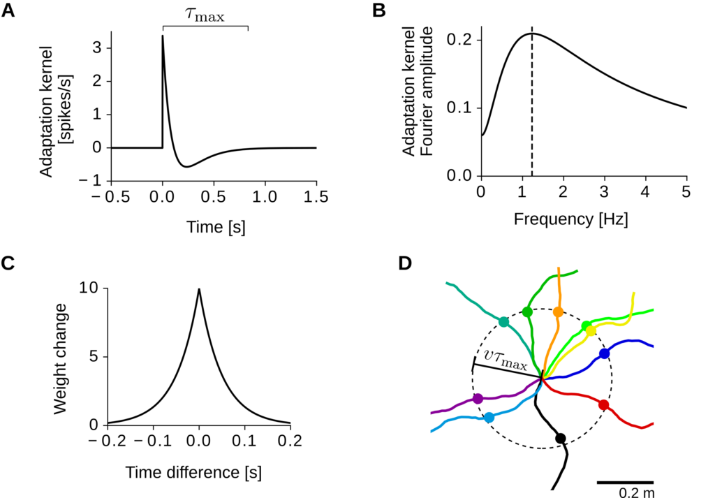
Model of grid-pattern formation. A) Spike-rate adaptation kernel. A positive peak is followed by a slow negative response. Note that the kernel is small for t > τmax. B) Frequency response of the adaptation kernel. The dashed vertical line indicates the kernel’s resonance frequency. C) Learning window for spike-timing dependent plasticity. The horizontal axis denotes the time difference between input and output spikes. D) Example virtual-rat trajectories (colored lines). All trajectories start at the center of the dashed circle and have a constant speed v. The colored dots mark the locations reached after a time τmax.
Figure 4 shows the results of one example simulation of this model. For clarity, we consider here the simplified scenario in which each input neuron i has a single Gaussian firing field at location ri and all locations are sampled evenly. In this case, the synaptic weights can be sorted according to the input firing-field centers ri and displayed in a 2D map (Figure 3A, top row). At the beginning of the simulation (t=0 s), all weights are initialized at random. However, as the virtual rat explores the arena, a symmetry breaking occurs: weights corresponding to close-by input fields grow together and several weight clusters emerge at a stereotypical length scale. Interestingly, such weight clusters – which set the locations where the output neuron fires – also tend to organize in a grid-like pattern.
We note that a triangular symmetry emerges after a substantial fraction of weights has hit the low saturation bound (at about t=2×10⁵ s in this simulation). Periodic pattern formation is indeed a strictly non-linear phenomenon, and excluding the spike generation process, weight saturation is the only non-linearity present in the system. In the linear regime, all Fourier modes at the critical spatial frequency exponentially grow with equal rate and independently from each other. In this case, the random weight pattern at time t=0 s is amplified at the critical frequency, but no periodic structure emerges. In the non-linear regime, instead, the exponentially growing modes are mutually coupled, and a second symmetry breaking occurs: only three Fourier modes with wave vectors that are 60 degrees apart survive (Figure 4 C, D).
In this model, the critical spatial scale of the patterns can be computed analytically and depends only on the temporal dynamics of adaptation, the size of the input firing fields, and the movement speed of the rat (D’Albis and Kempter, 2017). Additionally, the learning process is robust to random walks of variable speeds and to input spatial maps with multiple (randomly arranged) firing fields (D’Albis and Kempter, 2017).
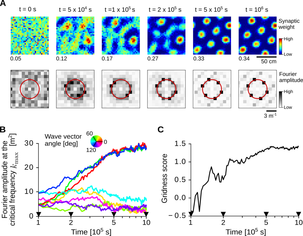
Simulation of the emergence of grid patterns.
A) Top row: evolution of the synaptic weights over time. Weights are sorted according to the two-dimensional position of the corresponding input receptive-field centers. Bottom row: Fourier amplitude of the synaptic weights at the top row. The red circle indicates the critical spatial frequency that dominates the dynamics. B) Time evolution of weights’ Fourier amplitudes at the critical frequency kmax. Wave vector angles (color coded) are relative to the largest mode at the end of the simulation. The black triangles indicate time points in C).
C) Gridness score of the weight pattern over time. The gridness score quantifies the degree of triangular periodicity.
Navigating with grid cells
I have presented a theoretical model in which grid-cell activity spontaneously emerges as result of a biologically plausible learning process. But how is grid cell activity used by animals to navigate? Although John O’Keefe and Edvard and May-Britt Moser were awarded the Nobel Prize in Physiology or Medicine for the discovery of “a comprehensive positioning system, an inner GPS, in the brain”, the role of grid cells in spatial cognition and navigation is far from being understood. Remarkably, most of place- and grid-cell data has been collected in contexts with minimal navigational demands, such as foraging in small featureless arenas, or running on straight linear tracks. By contrast, navigation in natural environments is a highly demanding task, which requires multiple sensory cues, cognitive strategies, and brain circuits.
From a theoretical point of view, grid-cell activity could provide two pieces of information to the animal: its current position in the environment, and its distance relative to a reference point or goal location (Herz et al., 2017).
But why should the brain represent space – a linear quantity – in periodic coordinates? Theoretical studies show that periodic multi-scale representations of space vastly outperform their unimodal counterparts, i.e., the range of distances that can be coded by a population of grid cells at different scales increases exponentially with the number of neurons N, whereas distances coded by place cells scale only linearly with N (Sreenivasan and Fiete, 2011). Remarkably, a handful of grid-cell populations (modules) with spacings ranging from tens of centimeters to a few meters could theoretically code distances up to several kilometers (Fiete et al., 2008; Stemmler et al., 2015) .
Grids beyond physical space
Grid cells have been largely studied in relation to animal location in physical space, but periodic neuronal representations are found in non-spatial contexts too. For example in rodents, grid cells represent distances in both space and in time (Kraus et al., 2015), and cells with periodic firing fields during locomotion often display multiple receptive fields in acoustic space (Aronov et al., 2017). In primates, entorhinal neurons show periodic tuning as a function of gaze location (Killian et al., 2012; Meister and Buffalo, 2018; Julian et al., 2018; Nau et al., 2018) and locus of attention (Wilming et al., 2018).
In humans, grid signals are observed during both virtual navigation (Doeller et al., 2010; Jacobs et al., 2013) and imagined navigation of the same paths (Bellmund et al., 2016; Horner et al., 2016), suggesting a role of grid-cell activity in trajectory planning and decision making. Finally, grid codes have been found to underlie abstract navigation in two-dimensional conceptual spaces (Constantinescu et al., 2016).
Altogether these studies suggest that grid patterns may represent behvioral variables that go far beyond the spatial domain. It will be exciting to see whether this line of research could provide further mechanistic insights into complex brain functions such as navigation, decision making, and abstract cognition.
References
Aronov, D., Nevers, R., and Tank, D. W. (2017). Mapping of a non-spatial dimension by the hippocampal–entorhinal circuit. Nature, 543(7647):719–722.
Bellmund, J. L., Deuker, L., Schröder, T. N., and Doeller, C. F. (2016). Grid-cell representations in mental simulation. eLife, 5:e17089.
Citri, A. and Malenka, R. C. (2008). Synaptic plasticity: multiple forms, functions, and mech- anisms. Neuropsychopharmacology, 33(1):18–41.
Constantinescu, A. O., O’Reilly, J. X., and Behrens, T. E. (2016). Organizing conceptual knowl- edge in humans with a gridlike code. Science, 352(6292):1464–1468.
D’Albis, T. and Kempter, R. (2017). A single-cell spiking model for the origin of grid-cell patterns. PLOS Comput. Biol., 13(10):e1005782.
Diehl, G. W., Hon, O. J., Leutgeb, S., and Leutgeb, J. K. (2017). Grid and nongrid cells in medial entorhinal cortex represent spatial location and environmental features with complementary coding schemes. Neuron, 94:83–92.
Doeller, C. F., Barry, C., and Burgess, N. (2010). Evidence for grid cells in a human memory network. Nature, 463(7281):657–661.
Fiete, I. R., Burak, Y., and Brookings, T. (2008). What grid cells convey about rat location. J. Neurosci., 28(27):6858–6871.
Giocomo, L. M., Moser, M.-B., and Moser, E. I. (2011). Computational models of grid cells. Neuron, 71(4):589–603.
Hafting, T., Fyhn, M., Molden, S., Moser, M.-B., and Moser, E. I. (2005). Microstructure of a spatial map in the entorhinal cortex. Nature, 436(7052):801–806.
Herz, A. V., Mathis, A., and Stemmler, M. (2017). Periodic population codes: From a single circular variable to higher dimensions, multiple nested scales, and conceptual spaces. Curr. Opin. Neurobiol., 46:99–108.
Horner, A. J., Bisby, J. A., Zotow, E., Bush, D., and Burgess, N. (2016). Grid-like processing of imagined navigation. Curr. Biol., 26(6):842–847.
Jacobs, J., Weidemann, C. T., Miller, J. F., Solway, A., Burke, J. F., Wei, X.-X., Suthana, N., Sperling, M. R., Sharan, A. D., Fried, I., et al. (2013). Direct recordings of grid-like neuronal activity in human spatial navigation. Nat. Neurosci., 16(9):1188–1190.
Julian, J. B., Keinath, A. T., Frazzetta, G., and Epstein, R. A. (2018). Human entorhinal cortex represents visual space using a boundary-anchored grid. Nat. Neurosci., 21:191–194.
Killian, N. J., Jutras, M. J., and Buffalo, E. A. (2012). A map of visual space in the primate entorhinal cortex. Nature, 491(7426):761–764.
Kraus, B. J., Brandon, M. P., Robinson, R. J., Connerney, M. A., Hasselmo, M. E., and Eichen- baum, H. (2015). During running in place, grid cells integrate elapsed time and distance run. Neuron, 88(3):578–589.
Kropff, E. and Treves, A. (2008). The emergence of grid cells: Intelligent design or just adap- tation? Hippocampus, 18(12):1256–1269.
La Camera, G., Rauch, A., Thurbon, D., Lüscher, H.-R., Senn, W., and Fusi, S. (2006). Mul- tiple time scales of temporal response in pyramidal and fast spiking cortical neurons. J. Neurphysiol., 96(6):3448–3464.
Meister, M. L. and Buffalo, E. A. (2018). Neurons in primate entorhinal cortex represent gaze position in multiple spatial reference frames. J. Neurosci., 38(10):2430–2441.
Moser, E. I., Roudi, Y., Witter, M. P., Kentros, C., Bonhoeffer, T., and Moser, M.-B. (2014). Grid cells and cortical representation. Nat. Rev. Neurosci., 15(7):466–481.
Nau, M., Schröder, T. N., Bellmund, J. L., and Doeller, C. F. (2018). Hexadirectional coding of visual space in human entorhinal cortex. Nat. Neurosci., 21:188–190.
O’Keefe, J. and Dostrovsky, J. (1971). The hippocampus as a spatial map. preliminary evidence from unit activity in the freely-moving rat. Brain Res., 34(1):171–175.
Sreenivasan, S. and Fiete, I. (2011). Grid cells generate an analog error-correcting code for singularly precise neural computation. Nat. Neurosci., 14(10):1330–1337.
Stemmler, M., Mathis, A., and Herz, A. V. (2015). Connecting multiple spatial scales to decode the population activity of grid cells. Sci. Adv., 1(11):e1500816.
Thue, A. (1910). Über die dichteste Zusammenstellung von kongruenten Kreisen in einer Ebene. J. Dybwad.
Tolman, E. C. (1948). Cognitive maps in rats and men. Psycholog. Rev., 55(4):189–208.
Wei, X.-X., Prentice, J., and Balasubramanian, V. (2015). A principle of economy predicts the functional architecture of grid cells. eLife, 4:e08362.
Wilming, N., König, P., König, S., and Buffalo, E. A. (2018). Entorhinal cortex receptive fields are modulated by spatial attention, even without movement. eLife, 7:e31745.
Zilli, E. A. (2012). Models of grid cell spatial firing published 2005–2011. Front. Neural Circuits, 6:16.